Why the Rich Can Get Richer by Sheer Dumb Luck

I’d long suspected that the rich tend to get richer, and not just because their larger wealth translates into more political influence and the capability to manipulate the system for their own benefit.  I wondered, suppose we could factor out all those other kinds of advantages that result from having more money, would it still be true that those with more money have an easier time gaining even more money, and conversely, would those with less money tend to lose even more of their limited funds?  I decided to do the experiment with a series of computer simulations to find out what happens.

And as you might suspect from the title, the result of the simulations shows that the rich do tend to get richer without even trying.  But the reasons might be surprising to you, and it is worthwhile trying to understand what is happening, so you can follow along here as I reconstruct what I did to explore this question.

Others have done similar studies, and what I have done is not particularly unique, though I hope you’ll find it helpful.  One in particular, “Follow the Money” by Brian Hayes (also in PDF), inspired me to dive into it and eventually write up what I found here.

The Simplified Simulated World

In each of these simulations, people will be represented very simply by the amount of money they have.  Each person will start out with the same amount of money, and we will run a simulation over several time steps, simulating changes of money that correspond to trades in the marketplace.  In each trade, when one person wins some amount, another loses the same amount, so the total amount of money always remains constant.   Unlike real trades where something else is typically traded in addition to the money, we are only considering the transfer of money.

Let’s also assume that, in this idealized world, everyone has an equal chance of winning or losing some amount in each trade.   This is not a realistic scenario in the real world, but it will be useful in these simulations to cancel out any kind of market knowledge or trading skill that either party might have that would give them an advantage.    (We also assume that the amount of a win or loss will usually be closer to zero rather than, for example, being evenly distributed over a range.  This probably doesn’t affect the outcome  but it will probably smooth the results.)

In the first simulation, everyone is treated equally, but in later simulations, we will modify the chance of winning or losing in each trade in various ways to find out what happens.

If we were to run a simulation in which each person randomly wins or loses up to a fixed amount, the same amount for each person, then there would be no difference between one person and the next, and there would be no significant difference in the changes from one time step of the simulation to the next.    (I didn’t even run such a simulation since the outcome is so obvious.)

But if, instead, each person can win or lose a random percentage of their wealth, the money they are holding at each time step, it turns out that this simple change will ultimately have a huge effect.  Remember that each person starts out with the same amount, so the same percentage will apply to each.  But after the first time step, after each person wins or loses some amount, each person will have a different amount of money, and therefore the same percentage of their current wealth will be different, which affects how much they can win or lose in the next time step.

To make this simulation simpler still, I decided not to simulate a sequence of individual trades directly between random pairs of people, where each trade results in a transfer of money one way or the other.  (Actually, I ended up implementing this variation later on.  See the section on”Trading with Each Other” below.)

Instead, I simply add or subtract a random amount from each person at each step of the simulation, keeping a running balance of the total excess or deficit, which we will call the Bank.  We can treat a win by one person as a cumulative loss by one or more other people, and vice versa.  Or we can think of this as trading via the intermediary of the Bank.  The Bank is never allowed to run a deficit with a negative value, so the size of trades is limited by what remains in the Bank during each trade.

Here (on the right) is a working program (written in Google’s Blockly language) that implements this simulation, though it is not exactly the same algorithm used to generate the visualizations below.  I show it here to make it clear that the simulation is rather simple.  I left out a few important details, such as how we need to randomize the order that each person gets to trade, but it’s basically the same idea.  (If you want to study how this works, I created an animation of the algorithm, which I’ll link to at the end.)

Equal Chance to Win or Lose

What would you guess will happen in this simulation?   Will the wealth of each person randomly rise or fall but stay about the same, even though people with greater wealth may win or lose larger amounts?  Will the money in the Bank stay close to zero (or whatever its original amount was)?

Quite honestly, I thought this simulation might show that a few people would accumulate most of the wealth which is lost by the rest.  But I wasn’t sure why that would be, or even if it would happen at all.  Finding out what would happen is exactly why I wrote the simulation.

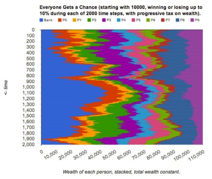
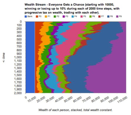
The following graph (on the right) shows the result of running this simulation one time.  Each color represents one person, P0 through P9, and the Bank is also represented on the left side of this graph using the color blue.  Each person, and the Bank, starts out with 10,000.  The width of each colored band represents the wealth of each person at each time step.  During each of 2000 time steps in this simulation, each person can win or lose up to 10% of their current wealth.

Notice that the Bank appears to be “winning” while everyone else eventually loses.  Each time we run this simulation, we will get different results.  Sometimes, it turns out, one or two of the people will get lucky for a while and increase their wealth.  But eventually, everyone’s luck runs out, and the Bank gets all the excess losses.

Why did this happen?  It was actually a surprise to me, and I thought it might be a bug in the simulation, until I checked it out and thought about it some more.

Percentage Change

Let’s walk through what happens if everyone has an equal chance of winning or losing a random percentage of their current wealth.  The number of times each person wins and loses will be about the same as for every other person, but the amounts will vary depending on the wealth that each person has at each time step.

What happens for one person? Imagine if you start with $100 and you gain 10% or $10; then you will have $110.  And if you then lose 10% of that, or $11, you will end up with $99, which is $1 less than you started with.  So after a win followed by a loss of the same percentage, you will end up with less than you started.

Here is a very nice and simple illustration of this concept of Percentage Change.

Example: 10% of 100

A 10% increase from 100 is an increase of 10, which equals 110 …

… but a 10% reduction from 110 is a reduction of 11 (10% of 110 is 11)

So we ended up at 99 (not the 100 we started with)

What happened? 10% took us up 10 Then 10% took us down 11 Because the percentage rise or fall is in relation to the old value: The 10% increase was applied to 100. But the 10% decrease was applied to 110.

But what happens if we do it in reverse, first losing and then winning?  Maybe you’ll come out ahead and everything will average out.  Starting with $100, if you first lose 10% or $10, you will have $90, and if you then gain 10% of that, or $9, you will end up with $99.  Again, you end up with $1 less than you started!

What does this mean?  After a random pair of trades, where you are likely to win or lose the same number of times, you are more likely on average to lose a small amount each time.  And once you have lost some of your wealth, it is that much harder to get it back since you are more likely to keep losing.  After a series of such random wins and losses of equal percentages, everyone, no matter how much wealth they start with, will most likely end up with less than they started.  That means that we should expect everyone to gradually lose, and the Bank will gradually take up all the excess that was lost.  Indeed, that is what we see in the simulation.

Changes in Wealth Distribution Over Time

It is fairly clear in the above graph that the wealth of each person is tending to decline.  But I want to introduce another way of looking at the data that will make it even more clear, and later, we can compare this to what happens when we change the rules.

If we divide up the whole time of the simulation into intervals, say 20 intervals of 100 time steps each, then we can look at what is happening during each time interval and compare that with the other intervals.  For each interval, we will list all the values of wealth that any of the 10 people has (not including the Bank) at any time during that interval, that will result in a list of 100 x 10 = 1000 samples.

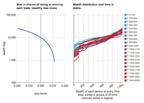
Then we can sort the list from lowest to highest and plot these points to give a good picture of the distribution of wealth during that interval, and we can repeat this for each interval.  The graph on the right shows what this looks like for the 20 intervals.  The earliest intervals in cyan show a relatively flat distribution compared to the later intervals in red.  The last lines show the wealth ranging from about 100 to 25,000.  Note that the wealth axis uses a log scale.

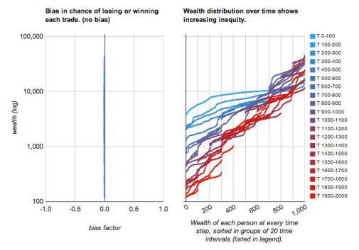
On the left is another graph that merely shows there is no added bias in the chance of losing or winning for each person no matter what their level of wealth is.   (Later, I will add some bias, to see what happens.)  But while there is no added bias here, what is the actual distribution of wins and loses?  Are the rich merely winning more often, or larger amounts?  To answer that, we will have to do some more analysis of the data.

Histogram of Loss or Gain

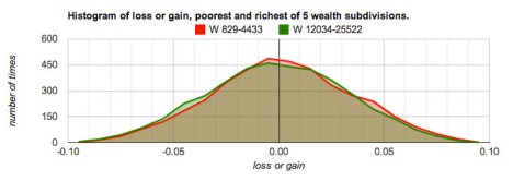
If we record all the changes in wealth of each person at every time step, sort them, and then group them into several buckets, one for each range of the amount of change, then we can plot the size of each bucket to get a histogram.  What we want to do is compare the poorest and richest groups of people to see whether there is any difference in the histogram of changes.  I divided all the change data into 5 equal-sized subdivisions based on the level of wealth so we can just look at the first and last subdivisions.  This comparison is easier to see using the area charts shown next.

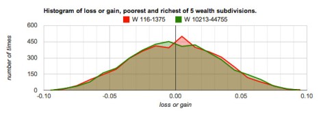
This shows that both the poorest (in red) and richest (in green) subdivisions have a similar distribution of losses and gains, except, curiously, close to zero.  The poorest are actually winning slightly more while the richest are losing slightly more.  Why would this be happening?  It does appear to be happening almost every time I run the simulation.  Again I thought it might be a bug in the simulation, but it might make sense given one of the rules I haven’t mentioned yet, that the amount of change is always rounded to a whole number.   For those with low wealth, a small percentage loss will tend to round up to zero.   In any case, this small advantage for the poor doesn’t seem to be helping them much, except for maybe keeping them from falling all the way to zero.

Redistribute the Excess

In the first simulation, we found that the Bank tended to accumulate all the losses of everyone else.  So what would happen if we merely redistribute this accumulated wealth?   There are several different ways this could be done, but I implemented it by simply dividing up the excess equally, so the amount each person gets is independent of their current wealth.  On the other hand, if the Bank has a deficit, then we can similarly extract an equal portion from each person.  As each trade occurs, the excess or deficit in the Bank changes immediately, which affects the redistribution that the next person might get.

With this change of the rules, you might think that this should even things out, since everyone has an equal chance of winning or losing.  In the first simulation, we found that everyone had a slight chance of losing, and the Bank ended up with the excess.  But now that the excess is being distributed a little at a time in each trade, this might cancel out the slight chance of losing.  But that is not what happens as you can see in the graph.

Notice that the Bank hovers around its initial value of 10,000, while one person, P2 in green, appears to be taking over the role of the Bank.  If we run this simulation several times, because the Bank is effectively prevented from growing, someone else always seems likely to accumulate most of the wealth lost by everyone else.   Sometimes more than one person will contend for the dominant position, for a while.

Why is this happening?

I don’t have a complete answer yet, and this is worth further study.  This result is what I was hoping the simulation would show, but now that it has, I’m still not sure exactly why it is happening.  Here are some possibilities to consider.  Anyone could win some portion of the Bank’s money with equal probability of winning or losing, and when they do win, everyone pays equally for the deficit. Similarly, when one person loses, everyone shares equally in the excess.  It must be the case that there is still a slight chance for everyone to lose, and since the bank can’t accumulate the excess, now it ends up in one (or a few) of the people.

This is the sheer dumb luck that I referred to in the title.   Even though everyone is treated “equally”, why do a few end up accumulating all the wealth while everyone else gets squeezed to almost nothing?  In this simulation, we distributed the excess equally, or so we thought, and we still ended up with inequity.   But consider what would happen if we distribute the excess in proportion to the current wealth of each person, rather than equal portions to each; it resulting inequity ought to be even worse.  (We should do that experiment just to be sure.)

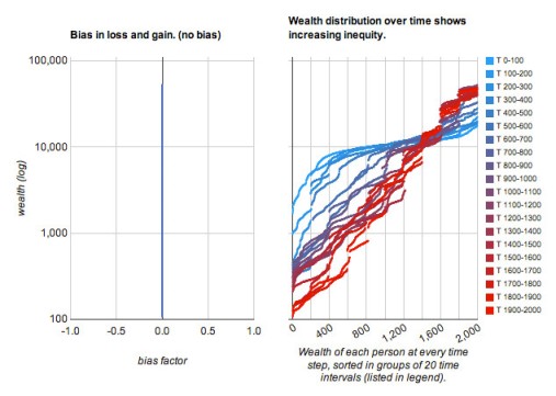
We can see the very extreme inequity in the distribution of wealth in the following graph on the right, ranging from about 300 to 80,000.

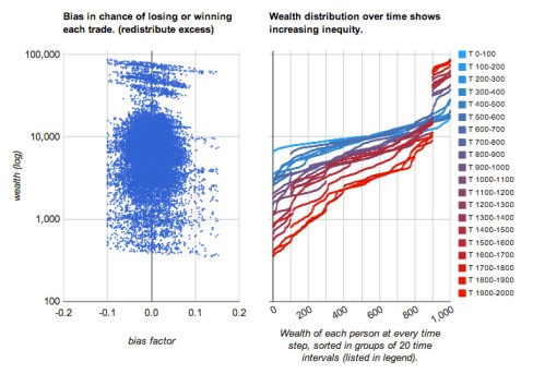
Compare the Wealth Distribution for this simulation with that of the first simulation, and you’ll notice that the main difference is that the wealthiest people get even more wealthy.  The discontinuities in the wealth distribution curves in the upper right reflect the growing wealth gap between the richest and everyone else.

Now the Bias graph on the left shows something more interesting than in the first simulation.   Each dot represents the bias that was computed for a particular person at some time step, not based on their wealth but only on the current excess in the bank.  There is only a very small amount of bias in the probability of winning and losing (plus or minus 1/10th of the 10% chance of winning or losing) that appears to be uniformly distributed at all levels of wealth.

Note a couple of interesting things about the Bias graph.   Overall, there appear to be a few dots further to the right (to the right of the 0.1 value) which suggests there is a slightly greater chance of winning for everyone.  This might be equivalent to the excess that would have otherwise stayed in the Bank, but it might just be an artifact of the calculations.

Also curious, there is a slight slope downward to the right that is especially visible at the highest levels of wealth.  This seems to be showing that the wealthiest have a slightly greater chance of losing in this simulation, actually, and perhaps it makes sense with a finite amount of total wealth because the wealthiest will have less chance of winning the little that remains.  But this same slope is visible at the bottom end of the wealth scale as well, and you can see traces throughout.  This needs further investigation.

If we look at the histogram of loss or gain, …

… we can see that it is fairly uniform except for a couple of bumps.  These bumps don’t always happen in the same place, however, and various other non-uniform things happen each time we run the simulation.  I suspect the growing accumulation of extreme wealth and poverty are contributing to the non-uniformity of the histograms.

Progressive Taxation with Redistribution

In the next simulation, I experiment with one way to avoid the extreme accumulation of wealth by a few.   I think it is fair to say that all ways of dealing with this inequity amount to taxing the wealthy more than the poor, but there are many ways that could be done.

I’ll keep it simple by just subtracting a fraction of the excess wealth that each person has relative to what they started with, and by similarly adding to those with a deficit.  So this is a wealth tax (and subsidy) rather than an income tax.

We are continuing to redistribute excess in the Bank, just as in the previous simulation.  So we are only adding this one rule that makes it harder for the rich to win and easier for the poor to win.

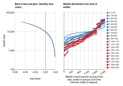
The pattern in the graph on the right seems clear – that everyone stays within a reasonable limit.  The Distribution of Wealth graph shows that there is a range of wealth that remains constant throughout the simulation, from about 5,000 to 15,000.  There is no hard upper or lower limit on the wealth of each individual, but the progressive tax takes care of keeping the extremes within this reasonable range.

The Bias graph shows that the bias required to achieve this result is not all that much, up to a maximum of about 1/10th of the 10% chance of winning or losing, just the same as for the redistribution.  The overall slant in the bias points shows how the higher levels of wealth (which is not very high this time) pays the hit of slightly more losses.

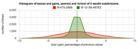
The Histogram of Loss or Gain makes it clear how this bias shifts the whole curve of the richest toward more losses, and the poorest toward more gains.

Progressive Tax Alone

Next, I wondered if the progressive tax alone could avoid the wealth gap and keep the extremes within bounds, while allowing excess losses to accumulate in the Bank. Also, I wondered how small the progressive tax could be and still do well enough to avoid crossing a threshold (if there is one) where the rich tend to keep getting richer to the limit of accumulating all wealth while everyone else is left with nothing.

In this simulation without redistribution, while the Bank might grow large at times, unlike in the first simulation, it doesn’t stay that way indefinitely because the poor are subsidized by the progressive tax, which also draws on the excess in the bank.

Consequently, the distribution of wealth has a wider range than it was in the previous simulation, but it rarely drops below about 1000 or rises above 25,000, and it appears relatively stable over time.

This time, I used a progressive tax that is only 1/5 of what is shown in the previous simulation, as you can see in the Bias graph.  Notice that the bias is grows the largest for the richest as compared to the poorest. (See the extension out to -0.032 in the upper left.)   It’s almost as if it is more difficult to keep the rich in check than to prop up the poor.

The curve in the Bias graph, by the way, is due to the log scale for the wealth axis.  If it were plotted on a linear scale, it would be a straight line.

The Histogram of loss or gain shows hardly any difference between the two groups, with slightly more losses for the richest and slightly more gains for the poorest.

Trading with Each Other

As I began to write up this report, I went back to reread other studies, especially “Follow the Money”, where a trading model is often used instead of relying on the Bank to act as an intermediary as I did.  And despite some added complexity, I decided to implement this option as well.

Similar to other studies, when two people are trading, the maximum that can be traded is limited by the one with less wealth. This means that those with the most wealth will be risking less in each trade, which implies (unless they have more opportunities to trade) that the rate of change in their wealth will be slowed, but it doesn’t affect the direction of that change.  So I was curious to find out what would happen.

During each time step, everyone gets to trade with another randomly picked person, and the order is also random, by the way.  So everyone gets to do at least one trade, and some might get one or more additional trades, if picked as the other person.  This means that during each time step, each person does two trades on average, so it is like running the simulation twice as long.

In the Wealth Stream graph (let’s call it) notice that the Bank stays constant this time.  In this particular run, two people, P7 and P9, are vying for dominance near the end of the 2000 time steps.   We are back to no progressive tax, by the way, so this is very much like the result of the Redistribution run, without the need to do a redistribution since the Bank doesn’t play a role.

The Wealth Distribution graph shows a similar growing inequity like what we saw in the first two simulations, with a range between 100 and 45,000, so it is just as bad on both ends, if not worse.

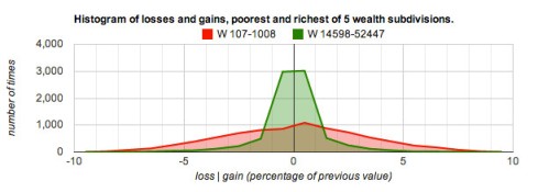
And the Histogram of loss or gain shows a large increase, for the wealthy subdivision, in the number of trades with loss or gain closer to zero, which is to be expected since the size of each trade is limited by the less wealthy of the two.

So this Trading simulation shows that my approximation of trading using the Bank as intermediary, along with redistribution of the excess, is not all that different in end result.   Also noteworthy is that the limitation on the richest traders to trade no more than what the poorer trader has available doesn’t stop them from accumulating all the wealth.

Trading with Progressive Taxation

Can we keep the inequity from growing in the Trading simulation by using progressive taxation just as we did when using the Bank as intermediary?  It turns out we can, though it is a little harder, it seems.

The Wealth Distribution graph is similar to that of the simulation of Progressive Tax Alone, but with higher highs, ranging between 1000 and 45,000.  The progressive tax is the same, but perhaps it is not quite enough here to keep the rich under control, although it keeps the poor from falling too far down.  This makes sense, however, because the bias is only computed relative to the less wealthy person in the trade (to keep it simple), and this means the wealthy don’t suffer this tax quite as much as they otherwise would.

We’d have to run it more times, or longer, to find out how stable it is.  I ran it a few times to 4000 steps and it doesn’t seem to get much worse, except occasionally, but the progressive tax always seems to pull the extremes back into line eventually.

The Histogram shows pretty much the same pattern.  Given the huge difference between the poorest and richest subdivisions in the trading patterns, it is difficult to compare the two beyond the obvious, nor can we compare with the previous run.

You might notice that I changed some of the labels in the graphs.  The “Histogram of losses and gains” now shows the “loss | gain” axis with percentages.   Feel free to make suggestions for other improvements.

(I fixed a bug that was visible in an earlier version of this blog, in case you saw that.  For the two Trading sections, the Distribution and Histogram charts were not showing the data for the other person in the trade, the more wealthy of the two.)

Conclusions?

I started out wanting to build my own simulation of trading, just to see for myself what happens.  I was hoping it would show what it appears to show, that the rich do tend to get richer purely by chance alone, if we ignore all the other ways they have advantages in the marketplace.  This series of simulations is not conclusive only because it is not a thorough study of the statistical significance of the results.  But it does strongly suggest that this is the case, and I hope it inspires a few more people to do some further study.

Another reason it is not conclusive is that I don’t quite understand and can’t explain the mechanism by which it happens.  It is clear why everyone has a slight chance of losing more than gaining, in a series of random trades of equal percentage of current wealth (see the section on Percentage Change).  But why do a few end up with the accumulated losses?  This seems to be an emergent effect, since the losses have to end up somewhere.  I’ll be thinking about more ways to analyze the data and other simulations to try to help me understand this, and I invite your suggestions.

I am considering adding an income tax option to compare that with the wealth tax.   I’m also probably going to add an optional “skill” bias to see whether skill is rewarded as we would like it to be and whether it is strong enough to contend with the random winner effect.

Another motivation was to use Google Charts in some interesting ways, partly to learn how well they work in practice and where they might fall short.   I’ve learned a lot about the challenge of getting the axes to show what I want, especially the log scale axis.

Try the Simulation Yourself

You can run the latest version of the simulation and change many of the parameters yourself by visiting the “full screen result” page or the “code editor” page.  At the bottom of both is an animation of the basic algorithm written in Python (which might be disabled when you go to look for it).  Also at epleweb.appspot.com

References

1. “Follow the Money” by Brian Hayes (also in PDF)
   
2. “Distribution of Monetary Wealth” by J.C. Sprott
3. “A computer simulation: Why the Rich get Richer and the poor – lose everything“
4. “Chance helps the rich get richer, simulation study finds”
   1. “Entrepreneurs, Chance, and the Deterministic Concentration of Wealth” by Joseph E. Fargione
5. “Concentration of Wealth Simulation“
6. “The Principle of Cumulative Advantage“